Introduction
This is an informal summary covering the testing of lp-CMFD with the Discontinuous Galerkin Finite Element Method, which we documented in the publication “A Linear Prolongating Coarse Megsh Finite Difference Acceleration of Discrete Ordinate Neutron Transport Calculation Based on Discontinuous Galerkin Finite Element Method” published in Nuclear Science and Engineering.
This post is a second part in a multipart series (Part 1, 3) covering the work that I did to test and develop lp-CMFD. Due to the length, this post is broken up into parts (a) covering 1D DGFEM and (b) covering 2D DGFEM (link). This post will cover the implementation of DGFEM discretization with CMFD and its variants. A more in-depth explanation of lp-CMFD is given in part 1 (specifically this section), which will not be repeated here for the sake of conciseness.
What is DGFEM
This series of publications demonstrate the coupling of lp-CMFD acceleration with DGFEM discretization of the neutron transport equation. The DGFEM method is a type of numerical method used to approximate the solution of partial differential equations (PDE) over cell meshes (the “finite element” part of the name). In DGFEM, each variable in a cell mesh is modeled as a linear combination of basis functions with unknown coefficients. Let us denote the number of basis functions as $N$. The solution of these coefficients is obtained by multiplying the PDEs (rewritten generally as $f(x) = 0$) with each basis function separately (the “Galerkin” part of the name1) and integrating over the mesh domain. Thus we obtain $N$ simultaneous equations with the unknowns being the coefficients of the basis functions ($\vec{c}$ of length $N$). We then cast the DGFEM equations as a matrix equation
$$
\boldsymbol{A}\vec{c} = \vec{b}
$$
and inverse the $M \times M$ matrix $\boldsymbol{A}$ to get $\vec{c}$
$$
\vec{c} = \boldsymbol{A}^{-1}\vec{b}
$$

Common choices of basis function sets are the orthogonal Legendre basis functions and the Lagrangian basis functions. The above table shows the forms of the basis function sets for 1D domains with spatial variable $x$ normalized between [-1, 1] Note that the number of functions in a set is controlled by the polynomial order $p$.

The corresponding Lagrangian points in 2D for triangle and square meshes. Note that the dots represent points where the Lagrangian basis set outputs 1. Also note that triangular and square meshes can be skewed, transformed or rotated with appropriate normalization methods.
There are several attractive features of DGFEM over other discretization methods:
- Variables are allowed to be discontinuous across mesh boundaries (the “discontinuous” part of the name)
- Flexibility of polynomial order and mesh adaptation. We can dynamically increase the number of basis functions and refine the mesh in regions where we sense that certain variables are changing rapidly
- The ability to handle complex mesh geometry
Implementation of DGFEM to the neutron transport equation
Detailing the implementation of DGFEM to the neutron transport equation and programming it in MATLAB is too involved for this post hence I will only highlight the main steps executed by the code.
Geometry and matrix preprocessing
- For each mesh, compute the DGFEM matrix based on the mesh geometry and the specific basis function for that cell.
- The convective nature of the neutron transport equation means that we can schedule the solution of the mesh cells by solving upwind cells first before downwind cells based on the direction of the angular flux $\psi$. The output from the upwind cells are used as inputs to the downwind cells. We determine the order using a Tarjan depth-first-search.
- Set initial flux and source distributions for the domain
Execution for $k$-eigenvalue Sn transport sweep with lp-CMFD acceleration
- Calculate fission and scattering sources using $\phi$ values
- For each angular direction, sweep through the domain starting from upstream meshes to downstream meshes, obtaining updated values of $\phi$ and $\psi$
- Use $\phi$ and $\psi$ as inputs to solve the diffusion equation on the coarse mesh basis and get the coarse mesh flux values $\Phi$
- lp-CMFD step: use $\Phi$ and $\phi$ and geometric interpolation to obtain the flux update parameter $\delta \phi$
- Update the flux $\phi \leftarrow \phi + \delta \phi$
- Repeat steps 1-5 until convergence is reached
Step 4 is the crucial step which we developed in order to implement lp-CMFD for DGFEM, so we can go into more detail on how this was calculated. We will start by defining the fine mesh flux averaged over the coarse mesh geometry as $\phi_{M}$ ($M$ is the coarse mesh index) which is calculated from the fine mesh flux $\phi_{m}$ ($m$ is the fine mesh index)
$$
\phi_{M} = \text{volume weighted mean }(\phi_{m}) m \in M
$$
We then denote the coarse mesh flux solved using the finite difference method as $\Phi_{M}$. The coarse mesh difference is $\delta\Phi_{M} = \Phi_{M} – \phi_{M}$. We repeat this procedure for every coarse mesh in the domain. We can calculate the $\delta\Phi_{M}$ values at the vertex of the coarse mesh grid. On the 1D domain the vertices of the coarse mesh grid are also the boundaries between neighboring meshes. The update value between coarse mesh $M$ and $M+1$ is the average between coarse mesh $M$ and $M+1$.
$$
\delta\Phi_{M+1/2} = \frac{1}{2}(\delta\Phi_{M} + \delta\Phi_{M+1})
$$
The vertex boundary values for coarse mesh $M$ is $\delta\Phi_{M-1/2}$ on the left and $\delta\Phi_{M+1/2}$ on the right. We can therefore linearly interpolate on the interior of the coarse mesh
$$
\delta\phi(x) = \delta\Phi_{M-1/2}(1 – \frac{x}{\Delta_{M}}) + \delta\Phi_{M+1/2}\frac{x}{\Delta_{M}}
$$
where $\Delta_{M}$ is the length of the coarse mesh and $x$ is the spatial coordinate between $[0, \Delta_{M}]$ within the coarse mesh. We can employ the DGFEM weighted residual method and find the updates to the coefficients. We will define the update flux in fine mesh $m$ on the same set of basis functions which was used in the $S_{N}$ transport calculation i.e.
$$
\phi^{update}(x) = \sum_{p} s_{p} u_{p}(x),
$$
where $s_{p}$ are the update coefficients of the basis functions $u_{p}$ to be solved. The residual equation is defined as
$$
\delta\phi(x) – \phi^{update}(x) = 0
$$
We generate $P$ number of equations by multiplying the residual equation with each basis function $u_{p}$
$$
\int (\delta\phi(x) – \phi^{update}(x)) \cdot s_{p}u_{p}(x) dx = 0 \text{ for } x \in x_{m}
$$
We skip the mathematical manipulation and simply cast the $P$ number of equations in matrix form
$$
\boldsymbol{T}\vec{s} = \vec{v}
$$
and finally
$$
\vec{s} = \boldsymbol{T}^{-1}\vec{v}
$$
We finally update the coefficients in fine mesh $m$ as
$$
\vec{c}^{update}_{m} = \vec{c}^{S_{N}}_{m} + \vec{s}
$$
Testing of lp-CMFD with DGFEM on 1D geometry
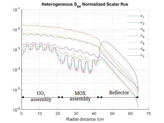
We tested our lp-CMFD update method for DGFEM on 1D geometry. We used as the basis of our test the time independent C5G7 problem (link). This problem is originally a 2D problem which we took a 1D slice of, and used the 7 group cross-sections from the benchmark. The problem consists of a UO2 assembly, a MOX assembly and a reflector assembly with reflective boundary condition on the left and vacuum boundary conditions on the right.

We solved the pin-resolved C5G7 problem and obtained the scalar fluxes (top), and then also spatially homogenized the structures to get assembly averaged 7-group XS parameters (bottom) for the subsequent tests.
We tested the effect of choice of angular quadrature i.e. by changing the value of $N$ in the $S_{N}$ transport problem, and its impact on relative performance between CMFD and lp-CMFD.

We can observe that lp-CMFD has a more effective acceleration than CMFD. We can also notice that the CMFD acceleration depends on the choice of angular quadrature set whereas lp-CMFD has the same performance.
We next test the effect of the choice of basis function set, Lagrange or Legendre and the max polynomial in the set, $p$, on the relative performance. Note that $p=1$ is linear order, $p=2$ is quadratic and $p = 3$ is cubic, now for the results …

… lp-CMFD consistently outperforms CMFD across basis function set type and polynomial order of the basis function.
Lastly, we test the effect of changing the # of coarse meshes in the homogenized C5G7 assembly problem. The larger the # of coarse meshes per assembly, the small the size of the coarse mesh.

We get quite interesting results comparing between lp-CMFD and CMFD. We note that for CMFD, the larger coarse meshes, corresponding to a smaller # of CM/assembly, leads to CMFD diverging. In fact, it is only when the #CM/assembly = 16 or 32, is when the CMFD solution can converge. On the other hand, lp-CMFD is shown to be convergent regardless of the # CM/assembly. This is very promising as it shows that even when the coarse meshes are very large, (and in some situations we want 1 coarse mesh per assembly), lp-CMFD can provide convergent results!
Continue on to part 2(b) where we carry out numerical analysis for DGFEM in 2D geometry. However, it may make sense to go to part 3 first to see how we extend lp-CMFD to non-rectangular meshes.
In summary…
We developed the method to apply lp-CMFD for DGFEM based $S_{N}$ neutron transport solvers. We key step, involving the method to update the coefficients for the basis function set on the fine mesh can be easily calculated using routines which already exist in DGFEM codes. Testing the lp-CMFD coupling with DGFEM on a realistic 1D problem showed that lp-CMFD in general had a better performance in terms of being more effective at acceleration the solution to convergence, as well as being stable under certain geometric configurations where CMFD became divergent.
I have obviously simplified the problem greatly. This method is also known as the method of mean weighted residues. For more thorough explanations I would recommend looking at the textbook “Discontinuous Galerkin methods for solving elliptic and parabolic equations: theory and implementation” (2019) by Beatrice Rivière.