Paper summary: Machine learning approach for predicting nuclide composition in nuclear fuel: bypassing traditional depletion and transport calculations
Introduction
This post is an informal summary of the paper “Machine learning approach for predicting nuclide composition in nuclear fuel: bypassing traditional depletion and transport calculations” published in Annals of Nuclear Energy in December 2024. In this work we presented a regression model to predict the nuclide composition of a fuel pin based on the depletion conditions of the fuel pin. Images in this post are taken from my SKC 2024 presentation (found here) and from the paper itself.
Motivation
The generation of cross-section libraries for the fuel pellet material depends on the composition of that fuel pellet. When the fuel is at fresh conditions i.e. before it is placed in the reactor, the cross-section libraries are straight-forward to calculate. However, one needs to update the fuel pin nuclide composition in the fuel pellet due to depletion in order to obtain accurate cross-section libraries at various points in the fuel cycle.

FGXS: Few group cross-section libraries, BOC: beginning-of-cycle, EOC: end-of-cycle
This need to perform depletion calculations means that the computational cost scales linearly with the required depletion level. In certain computational problems, it would be useful to replace this tedious depletion calculation with an approximate solution generated by a pre-trained model. Essentially, we are creating a regression model which can predict the fuel pin nuclide evolution based on its depletion history (the conditions experienced by the fuel pin during depletion e.g. the fuel temperature, power level, moderator density etc.).
Such a model will have other uses beyond its application in accelerating cross-section library generation, such as:
- Time-critical source term release in severe accident analysis
- Spent fuel dosage estimation
- Breeder/minor actinide burner operation optimization
Recurrent neural networks and preliminary analysis
The change in the nuclide composition of the fuel pellet material is described by the Bateman equations, a series of coupled rate equations which includes terms due to nuclear transmutation, fission product yields, decay chains etc. Using matrix notation, we can write it as
$$
\frac{d\boldsymbol{N}}{dt} = \boldsymbol{A}\boldsymbol{N},
$$
where $\boldsymbol{N}$ is the nuclide concentration vector and $\boldsymbol{A}$ is a square matrix. We should note that $\boldsymbol{A}$ is dependent on several historic parameters e.g. the power of the fuel pin during the depletion, the fuel temperature and $\boldsymbol{N}$. How to solve the Bateman equation is not of interest to us and we simply denote the true solution of the equation with a function , $f$, as
$$
\boldsymbol{N}(t + \Delta t) = f(\boldsymbol{N}(t) , \boldsymbol{H}(t)),
$$
where $\boldsymbol(H)(t)$ is the historic state parameters held constant between $t$ and $t + \Delta t$ (we set $\Delta t = 10 $ days). In this work, our goal is to substitute the true function $f$ with a recurrent neural network (RNN) based model denoted by $g$
$$
\boldsymbol{N}(t + \Delta t) \approx g(\boldsymbol{N}(t) , \boldsymbol{H}(t)).
$$
The RNN model works by predicting $\boldsymbol{N}(t_{1})$ using information from $\boldsymbol{N}(t_{0})$, and subsequently using $\boldsymbol{N}(t_{1})$ to predict $\boldsymbol{N}(t_{2})$ and so on. The schematic can be seen below:
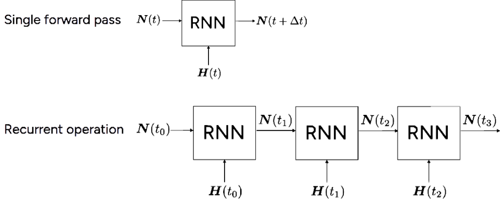
Single forward pass of the neural network to predict $N(t + \Delta t)$ (top) and the recurrence mode RNN operation where the outputs are re-fed as the network inputs (bottom)
Neural network objective function and training
The “training” of any neural network or regression model is the process of optimizing the model weights ($w$) by minimizing (or maximizing) some objective function. Very early on the process, we attempted several variations of the model objective function, and finally settled on two promising variants, which we termed the “Direct model” and the “Difference model”.
For the “Direct model”, the neural network directly predicts $\boldsymbol{N}(t_{1})$. The objective function for this model to be minimized is the mean squared error on $\boldsymbol{N}(t + \Delta t)$
$$
\mathcal{L}_{\text{direct}} = \frac{1}{I} \sum_{i}^{I} (N_{i}^{\text{Direct}}(t + \Delta t) – N_{i}^{\text{Ref}}(t + \Delta t))^{2},
$$
where $i$ is the sample index and $I$ is the total number of samples.
The alternative model which we were interested in is the “Difference model”. Unlike the Direct model, the difference model predicts the change in nuclide concentrations, i.e.
$$
\Delta \boldsymbol{N}^{\text{Diff.}}(t) = g_{\text{Diff.}}(\boldsymbol{N}(t), \boldsymbol{H}(t)),
$$
and then we perform simple addition to obtain $\boldsymbol{N}^{\text{Diff}}(t + \Delta t)$
$$
\boldsymbol{N}^{\text{Diff}}(t + \Delta t) = \boldsymbol{N}(t) + \Delta \boldsymbol{N}^{\text{Diff.}}(t).
$$
The corresponding objective function for the Diff. model is
$$
\mathcal{L}_{\text{direct}} = \frac{1}{I} \sum_{i}^{I} (\Delta N_{i}^{\text{Direct}}(t + \Delta t) – \Delta N_{i}^{\text{Ref}}(t + \Delta t))^{2}.
$$
The motivation behind the Diff. model is that since we are modelling fuel depletion, it is natural to perform regression on the decrease in U-235 composition and the accumulation of fission products in the fuel pellet material.
Preliminary error analysis and need to increase model robustness
We performed a preliminary test of the Direct and Diff. models by generating training data and implementing the models on Tensorflow. We quickly discovered that the RNN errors are much greater at the end-of-cycle (i.e. when the fuel pin is heavily depleted) compared to the beginning-of-cycle and that these errors were much larger than the training error. This was due to the fact that the recurrent nature of the RNNs mean that errors which occur upstream are propagated downwards.

In recurrence mode operation, errors ($\epsilon(t)$) upstream propagates downstream. This generally leads to a greater error after a couple of rounds of recurrence than near the beginning.
These propagated errors can cause the RNN predictions to fail in several ways. (1) we noticed that there was the tendency to have exponential growth in error terms related to order-of-magnitude changes in $\boldsymbol{N}$ especially for trace isotopes. The initial concentration of trace isotopes is $\sim 10^{-20}$ but can increase by several orders of magnitude. This is difficult, but not impossible, for the neural network to handle. (2) It was possible for the RNNs to predict negative concentrations for the nuclides. This is obviously an unphysical prediction. A combination of (1) and (2) leads to erroneous inputs which can be very far outside of what was in the training data set. We therefore needed to formulate a method which can increase the robustness of the model while avoiding the need to generate more training data.
$\alpha$-blend model
Another important observation that we made (and is in fact the reason why we found it interesting enough to publish in a paper), is that different nuclides had different prediction accuracies between Direct and Diff. RNN models.
Diff. model had better performance for U-235
We noticed that for U-235, the Diff. model had better performance than the Direct model. Below shows the histogram of $\Delta N_{U235}$ prediction for the Direct model. In a small fraction of predictions, the Direct model predicted positive $\Delta N_{U235}$, which is unphysical considering that U-235 should always be decreasing in the context of fuel depletion.
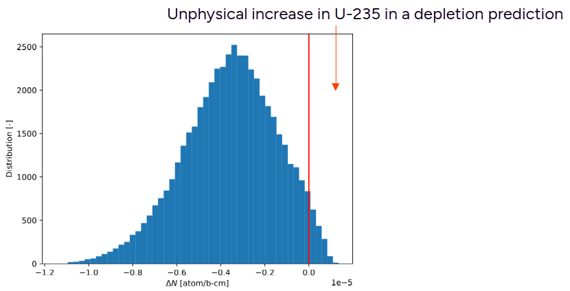
In Direct model, a small percentage of the time, U-235 concentration is predicted to increase, which is of course not possible in a fuel material
On the other hand, the Diff. model never predicted a positive $\Delta N_{U235}$:
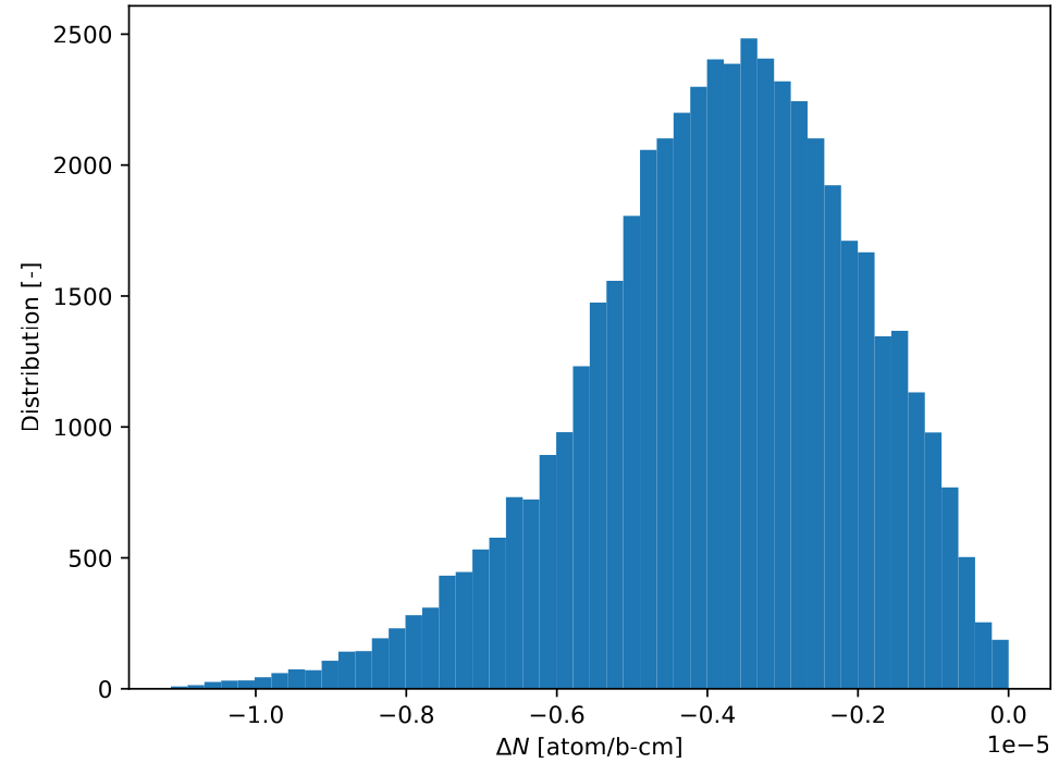
In Diff. model, there are no U-235 predictions which are increasing. This is because no such positive $\Delta N_{\text{U235}}$ is learnt from the training data, naturally constraining the output of the model.
Direct model had better performance for Xe-135
Xe-135 is a very important fission product for nuclear engineers due to its large absorption cross-section in the thermal energy range. It also has a relatively short (in terms of a power cycle) half-life of 9.2 hours. This means that if a depletion interval is long enough (in the order of days), then Xe-135 reaches equilibrium (i.e. the level at which the rate of Xe-135 production is equal to its removal). This state is even given special terminology in many depletion codes as “equilibrium xenon”, since it has such a large effect on the $k_{\text{eff}}$ of a reactor at start-up. Consequently, the Xe-135 concentration at the end of the depletion step (where $\Delta t = 10$ days) is almost independent of the initial Xe-135 concentration. This fact explains why we noticed that Xe-135 predictions had a better accuracy when using the Direct model compared to the Diff. model as shown below:
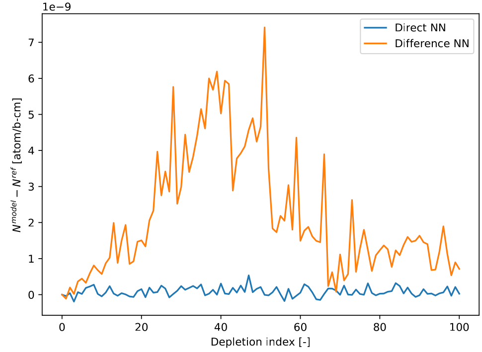
Comparison of the performance of Direct and Diff models for Xe-135 on test data. The Direct model performs much better.
Linear blending of Direct and Diff. models with optimization
Our observations thus far show that different models work better for different nuclides, and we also realised that there was no reason to force all nuclides to be on the same model! In fact, there was no reason why we can’t blend the outputs of Direct and Diff. RNN models with a blending parameter ($\alpha$) which is unique for each nuclide.
$$
N^{\alpha}_{m}(t+\Delta t) = \alpha_{m} N^{\text{diff}}_{m}(t+\Delta t) + (1-\alpha_{m}) N^{\text{direct}}_{m}(t+\Delta t),
$$
where $\alpha_{m}$ is the blending parameter for nuclide $m$. The optimization of $\alpha_{m}$ is not an easy task. Hand-tuning the individual $\alpha_{m}$ values is tedious and prone to error. Additionally, for “famous” nuclides such as U-235 and Xe-135 the values of $\alpha_{m}$ are easy to select, but for other nuclides it is much harder to intuit what the appropriate value of $\alpha_{m}$ should be.
We therefore came up with a method to select $\alpha_{m}$ values by treating it as an optimization problem with the following loss function i.e. select values of $\alpha_{m}$ so that the function is minimized:
$$
L_{m} = L_{N}(\alpha_{m}) + L_{\Delta N}(\alpha_{m})
$$
$$
L_{N}(\alpha_{m}) = \frac{1}{I \times \sigma_{N,m}} \sum_{i}^{I} [{N}^{\text{ref}}_{i,m} – (\alpha_{m} {N}^{\text{Diff}}_{i,m} + (1-\alpha_{m}) {N}^{\text{direct}}_{i,m})]^{2}
$$
$$
L_{\Delta N}(\alpha_{m}) = \frac{1}{I \times \sigma_{\Delta N,m}} \sum_{i}^{I} [{\Delta N}^{\text{ref}}_{i,m} – (\alpha_{m} {\Delta N}^{\text{diff}}_{i,m} + (1-\alpha_{m}) {\Delta N}^{\text{direct}}_{i,m})]^{2},
$$
where $\sigma$ represents the standard deviation in order to scale the relative magnitudes of $L_{N}(\alpha_{m})$ and $L_{\Delta N}(\alpha_{m})$. ${N}^{\text{Diff}}_{i,m}$ represents the RNN predicted depletion chain, $[\boldsymbol{N}(t_{1}), \boldsymbol{N}(t_{2}), \boldsymbol{N}(t_{3}) … ]$ given only the initial concentration ($N(t_{0})$) and the historical conditions. These equations basically mean that we want to optimize $\alpha_{m}$ such that the $N$ and $\Delta N$ error are both decreased.
Results
The $\alpha$-blend model was shown to increase prediction accuracy for many nuclides, showing that the method increased the robustness of the predictions with the same set of training data. We show the Mean Absolute Relative Error (MARE) for select nuclides in the following table.
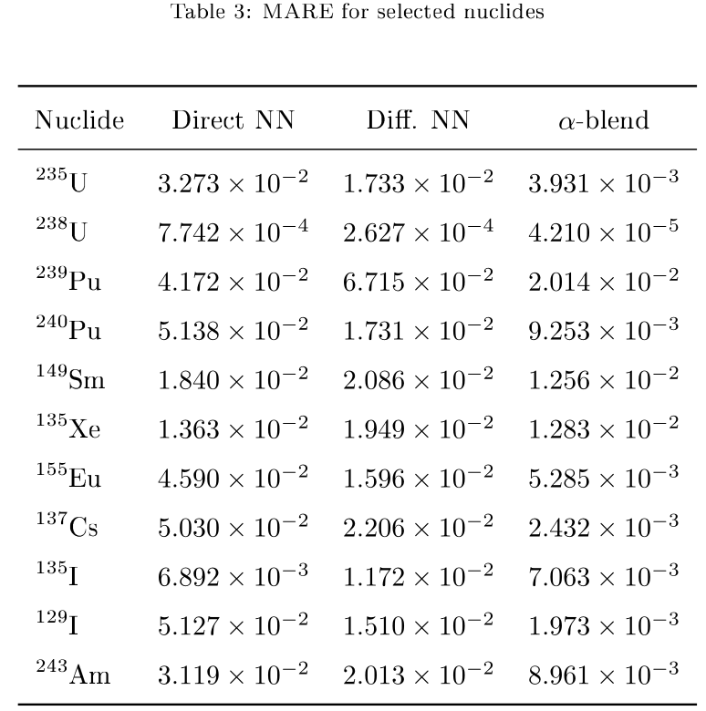
The $\alpha$-blend model is around one order of magnitude more accurate than either the Direct and Diff. NN models alone. We next examined whether the optimized $\alpha$-values met our expectations (recall that we expect $\alpha_{\text{U235}}$ is 100% Diff. model and $\alpha_{\text{Xe135}}$ is 100% Direct model).
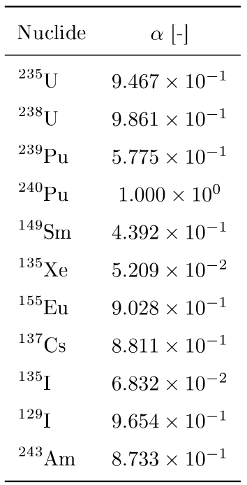
We obtained $\alpha_{\text{U235}} = 0.9467$ i.e. almost 95% of the output is from the Diff. model for U-235 and only 5% is from the Direct model output. For Xe-135, we had $\alpha_{\text{Xe135}} = 0.05209$, i.e. only 5% of the Diff model output is used for Xe-135 and 95% of the output is from the Direct model. Our method of optimizing $\alpha$ values automatically chooses values which meet our expectations and automatically chooses the right proportion of blending between the two models for each nuclide.
We also examined the behavior of the model in predicting $\Delta N_{\text{U235}}$.
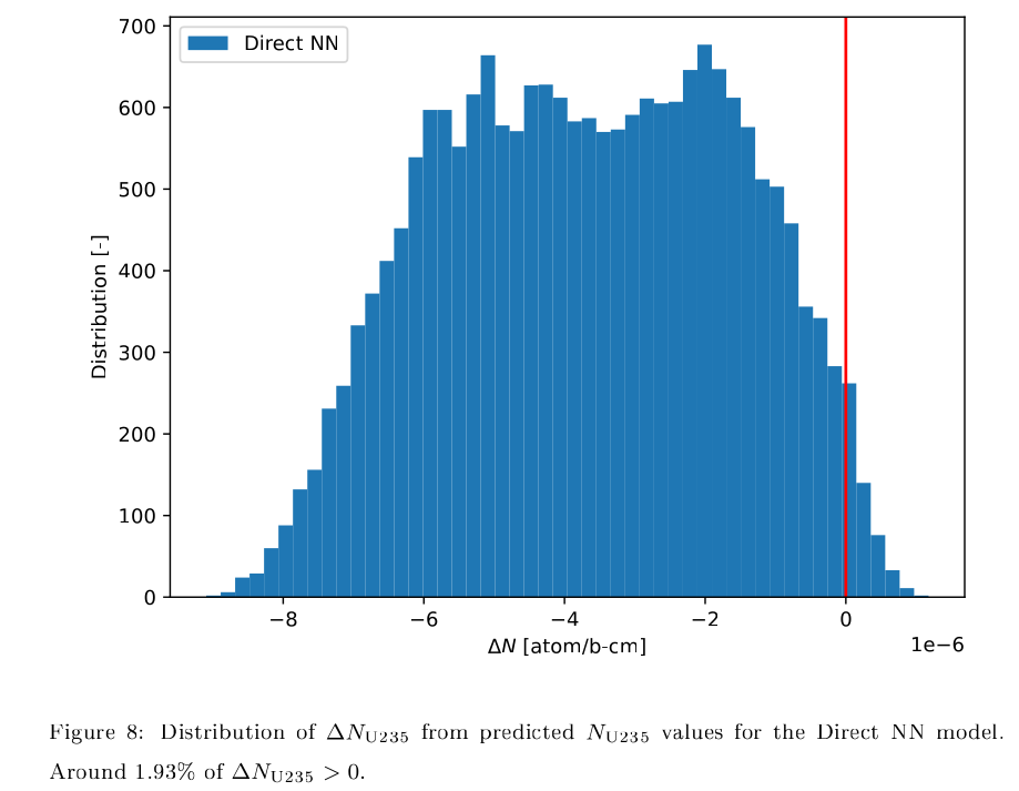
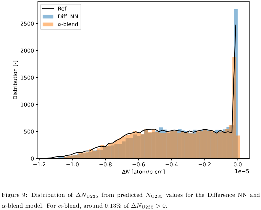
The $\alpha$-blend model has a much smaller percentage of $\Delta N_{\text{U235}}$ which are positive compared to the Direct NN model. Ideally, we would like this percentage to be 0 for $\alpha$-blend, but this is a problem for another day!
In summary…
We proposed a model which blends the outputs of two neural networks (which have different loss functions) with a nuclide specific blending parameter $\alpha$. These $\alpha$-values are automatically optimized by a minimization of a loss-function to avoid the tedium of hand-tuning these parameters. The obtained values met our expectations of what the optimal values of $\alpha$ should be (for U-235 and Xe-135). We showed that this improved model had higher accuracy and robustness compared to the separate neural networks alone. This was really good as we were able to improve the accuracy of the regression model without having to generate additional training data (which is computationally expensive).

